How to Move Grand Total to the Top in Pivot Table Using Power Query In Excel
Ever felt stuck because Excel puts the Grand Total row at the bottom of a Pivot Table and there’s no built-in way to move it to the top? You’re not alone. This is one of the most common layout frustrations Excel users face, especially in Excel 2019. If you’re trying to move grand total to top in pivot table for improved readability and a cleaner report, this limitation can quickly become a real obstacle.
In this guide, you’ll learn exactly how to move grand total to top in pivot table using Power Query. This isn’t a hack or gimmick. It’s a clean, dynamic, and refreshable solution that works every time. We’ll break down every step you need to take, including hidden steps and real roadblocks that you won’t find in most tutorials.
Why Can’t You Move the Grand Total to the Top in Excel by Default?
Microsoft Excel doesn’t natively support reordering the Grand Total row in Pivot Tables. The Grand Total is always calculated by default and placed at the bottom. There’s no drag option, no setting to flip it.
So, if you’re asking:
“How can I show Grand Total at the top of a Pivot Table in Excel 2019?”
The honest answer is: you can’t do it with built-in Pivot Table settings. But you can do it using Power Query. And that’s how we’ll help you move grand total to top in pivot table with a method that stays dynamic and accurate.
What You’ll Learn in This Guide
- How to create product-wise Grand Total rows manually using Power Query.
- How to position those rows at the top of your Pivot Table.
- How to structure the data for dynamic updates.
- How to fix Excel’s quirks like missing Append options and unwanted row labels.
- The easiest way to move grand total to top in pivot table without complicated formulas.
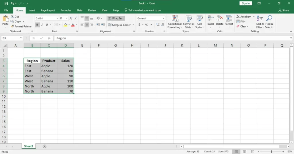
Step 1: Prepare Your Dataset
Create your data table like this:
| Region | Product | Sales |
| East | Apple | 120 |
| East | Banana | 80 |
| West | Apple | 90 |
| West | Banana | 110 |
| North | Apple | 100 |
| North | Banana | 70 |
- Select your data.
- Go to Insert > Table and confirm “My table has headers.”
Tip: Name your table for easier tracking in Power Query.
This structured format is crucial if you want to move grand total to top in pivot table later without breaking your data flow.
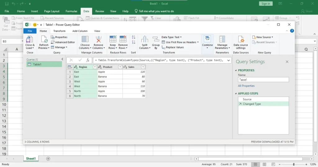
Step 2: Load the Data into Power Query
Go to Data > From Table/Range almost on the extremes left.
- Ensure “My table has headers” is checked.
- Click OK — Power Query Editor opens.
- You should now see your dataset loaded.
Using Power Query here is key to achieve the flexibility required to move grand total to top in pivot table the right way.
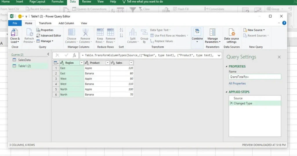
Step 3: Duplicate the Query
We need two versions of the data:
- The original table: SalesData
- A copy we’ll use to create a Grand Total row: GrandTotalRow
- In the Queries pane (left side), right-click on the query name.
- Click Duplicate.
- Rename the queries:
- SalesData
- GrandTotalRow
Hidden Step: Most tutorials skip explaining why you need a duplicate — this is necessary because you’re building a calculated summary (Grand Total) separately from the raw data.
This duplication is a small but powerful move if you’re committed to cleanly and best way to move grand total to top in pivot table.
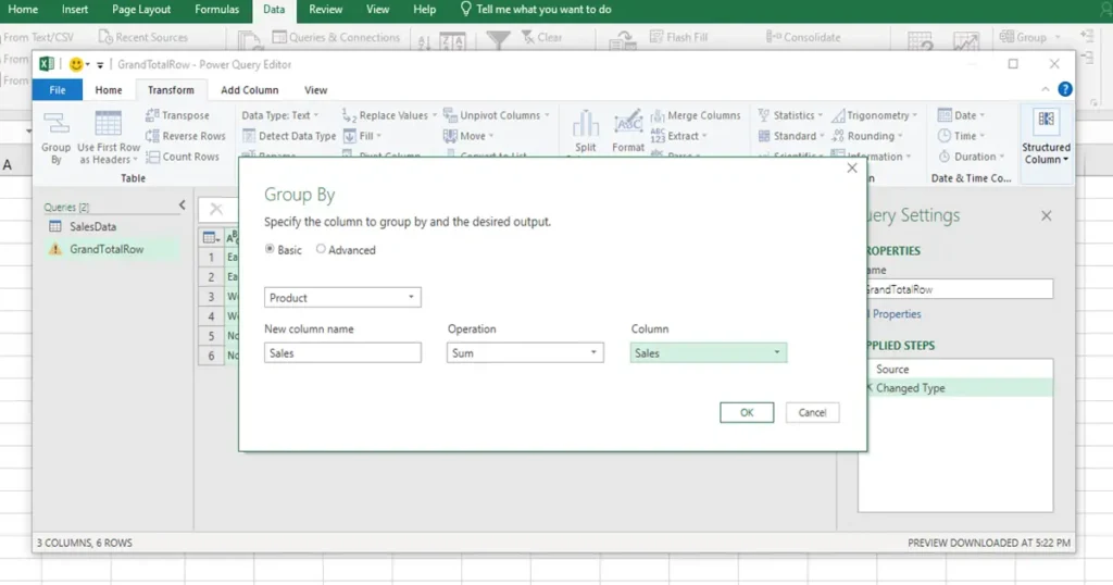
Step 4: Group the Data to Create Product-Wise Grand Totals
Now we build the Grand Total rows per product.
- Go to the GrandTotalRow query.
- Click Transform > Group By.
- In the dialog:
- Group By: Product
- New Column Name: Sales
- Operation: Sum
- Column: Sales
Hidden Insight: If you forget to group by Product, you’ll get one single row (e.g., 570), which won’t work for our Pivot Table.
This grouping technique gives us control to later move grand total to top in pivot table while keeping the breakdown intact.
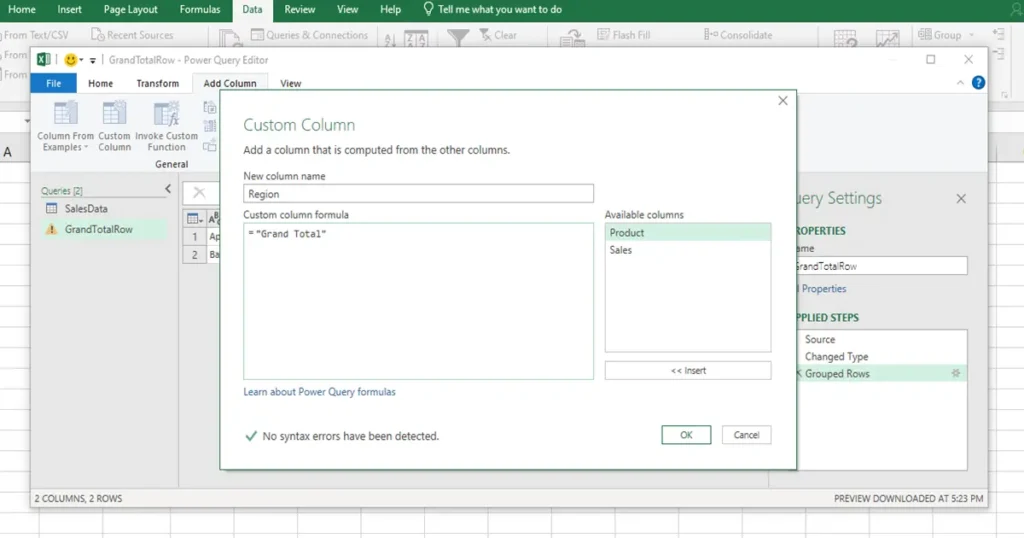
Step 5: Add Region Column to Label It as Grand Total
We now label our Grand Total rows properly.
- Go to Add Column Tab > Custom Column.
- Name: Region
- Formula:
- =”Grand Total”
- Click OK.
Pro Tip: Add this column after grouping. Adding it before causes Group By to re-aggregate the wrong way.
This label is what helps your Pivot Table recognize totals and helps us organize them cleanly when we move grand total to top in pivot table.
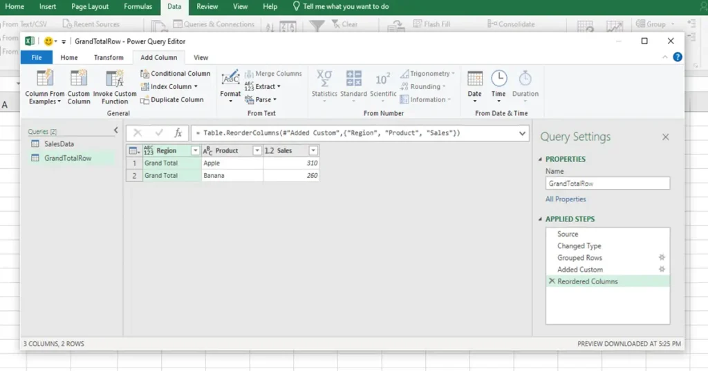
Step 6: Rearrange Column Order to Match
Ensure your final column structure looks like this:
| Region | Product | Sales |
| Grand Total | Apple | 310 |
| Grand Total | Banana | 260 |
If not, just drag columns into place inside Power Query.
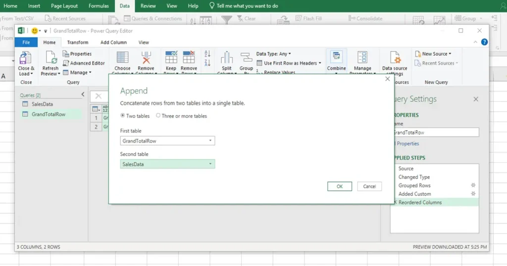
Step 7: Append Queries (GrandTotal + Original Data)
Now let’s combine everything:
- Go to Home (in power query editor) > Append Queries > Append Queries as New.
Hidden Step: In Excel 2019, “Append Queries” may be hidden under a “Combine” dropdown. If you don’t see it, expand your window or use the drop-down arrow.
- Choose:
- First Table: GrandTotalRow
- Second Table: SalesData
- Rename this query to FinalSalesData
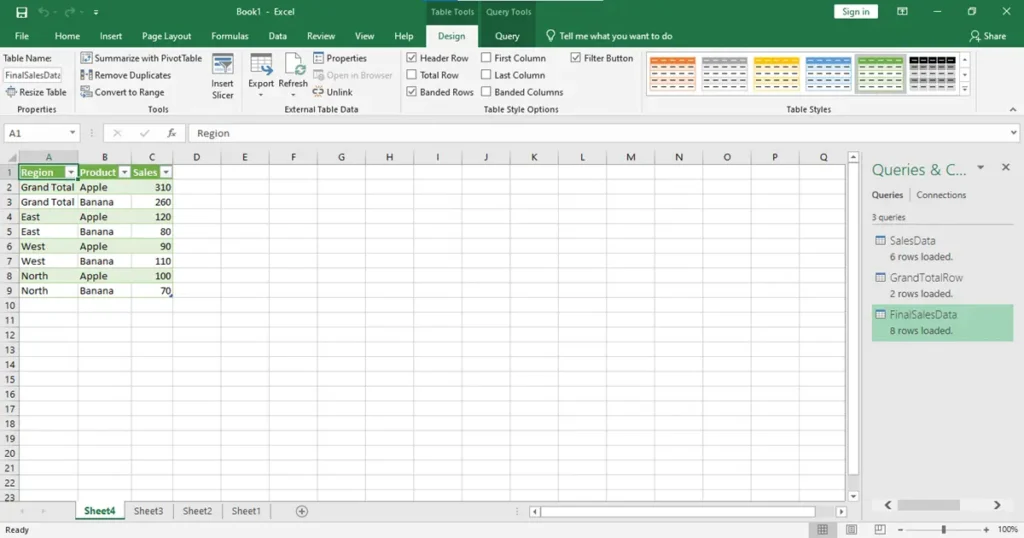
Your combined table should now show:
| Region | Product | Sales |
| Grand Total | Apple | 310 |
| Grand Total | Banana | 260 |
| East | Apple | 120 |
| East | Banana | 80 |
| West | Apple | 90 |
| West | Banana | 110 |
| North | Apple | 100 |
| North | Banana | 70 |
This append step is crucial when trying to dynamically move grand total to top in pivot table.
Step 8: Load Final Data Back to Excel
- With FinalSalesData selected, click Home > Close & Load To… (extremes left)
- Select Table > New Worksheet
- Click OK
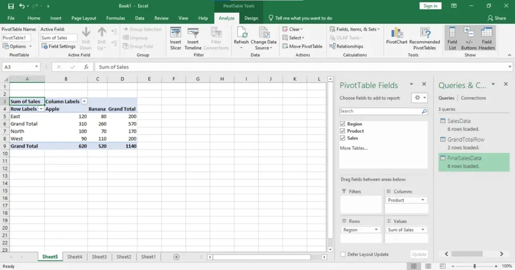
Now you have a clean dataset with Grand Totals at the top.
Step 9: Build the Pivot Table
- Select the FinalSalesData table.
- Go to Insert > Pivot Table
- Choose New Worksheet
- In the Pivot Table Field List:
- Rows: Region
- Columns: Product
- Values: Sales
This is where your effort pays off — you’ll now see a Pivot Table with Grand Total at the top. If this is on the second then right click Grand Total and click move and moves up. Yes, you’ve finally managed to move grand total to top in pivot table.
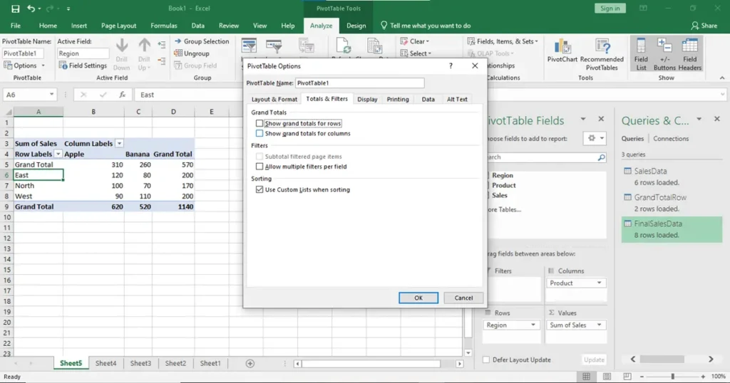
Step 10: Clean Up Pivot Table Layout
10.1: Remove Built-in Grand Totals
- Click inside the Pivot Table.
- Go to PivotTable Analyze > Options
- Under Totals & Filters:
- Uncheck:
- Show grand totals for rows
- Show grand totals for columns
- Uncheck:
10.2: Rename Row Labels to “Region”
- Click on the “Row Labels” header cell.
- Rename it to Region
Hidden Fix: Excel shows an annoying green triangle and blue “Row Labels” text unless you manually rename it.
Step 11: Automate Refreshing (Optional but Recommended)
Auto-refresh Query
- Open the Queries & Connections pane
- Right-click FinalSalesData > Properties
- Check:
- Refresh data when opening the file
- Refresh every 60 minutes (optional)
Auto-refresh Pivot Table (Macro Required)
Press Alt + F11 to open VBA Editor:
Private Sub Workbook_Open()
Dim pt As PivotTable
Dim ws As Worksheet
ThisWorkbook.RefreshAll
Application.Wait Now + TimeValue(“00:00:02”)
For Each ws In ThisWorkbook.Worksheets
For Each pt In ws.PivotTables
pt.RefreshTable
Next pt
Next ws
End Sub
Save the file as .xlsm
Conclusion
So, can you move the Grand Total to the top in Excel Pivot Tables? Technically, Excel doesn’t allow it directly — but there are a few smart workarounds.
Using Power Query is the most dynamic and reliable method. You could also use manual rearrangement or helper columns as simpler alternatives. However, only Power Query provides a fully automated and refreshable solution without relying on formatting hacks or manual edits.
If you’re looking for the most future-proof and professional approach to move grand total to top in pivot table, this Power Query method is it.
You’ve learned:
- How to use Power Query to group and label your totals
- How to combine custom total rows with original data
- How to automate updates and clean up Pivot layouts
If this guide helped, share it with someone who uses Excel daily!
For more practical tech tutorials, visit HassuTech.com or follow @HassuTech421 on Instagram.
FAQ’s
Q: Will this method work in Excel 2021 or Office 365?
Yes, this method to move grand total to top in pivot table works perfectly in Excel 2016, Office 365, and Excel 2021. All of these versions support Power Query, which is essential for implementing this technique smoothly.
Q: Can I do this without Power Query?
No, not dynamically. You would need to manually insert rows above the Pivot Table and label them accordingly. This approach is static and requires manual updates whenever the source data changes.
While it’s a possible workaround, it lacks automation and defeats the purpose of using a Pivot Table for dynamic reporting. Therefore, using Power Query is the recommended method to consistently move grand total to top in pivot table with better control and efficiency.
Q: Will my Grand Total update if I change the source data?
Yes, your Grand Total will update automatically if you enable auto-refresh, or you can refresh it manually when needed. This ensures your Pivot Table reflects the most recent changes in the source data without additional effort.
Moreover, this dynamic update maintains accuracy, especially if you’re trying to move grand total to top in pivot table while keeping it automated. As a result, your report stays current and eliminates the need for repetitive adjustments.


2 thoughts on “Excel Trick to Move Grand Total to Top in Pivot Table Automatically”
Сильная рассказ, лично пару дней назад штудировал
по вопросу??
you’re really a good webmaster. The web site loading speed is amazing. It seems that you are doing any unique trick. In addition, The contents are masterwork. you’ve done a wonderful job on this topic!